
Identifying redundant edges in a dependency graph
An ETL import graph is build on logical dependencies of the jobs to each other. So typically a SQL transformation job depends on all the previous jobs that create the tables used in the query. But once there are a certain number of jobs, dependencies often get a bit more complicated and some of them become redundant in the process.
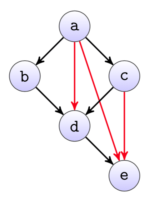
A simple example can be seen in the dependency graph from figure, where the three red edges are redundant. While they logically are probably still correct, they typically cause the graph layout to be way more confusing than necessary.
Yet it is not always that easy to manually find all the redundant edges. Therefore we automatically highlight them in our dependency graph, similar as in the example here.
Technically what we do here is to calculate the transitive reduction of the directed dependency graph. Since the graph is also acyclic, we can do this by using the well-known Floyd-Warshall algorithm.
The idea is to calculate all longest paths from any node to another within the graph (with all edge weights set to 1). If there is then an edge where the longest path between the nodes is greater than 1 (the edge itself), we can say the edge is redundant.
This can be seen i.e.\ for the redundant edge a -> d in the example graph. The longest path from a to d is 2, either through nodes b or c. Therefore d does not need the direct dependency to a, as it is implicitly given by
a -> b -> d or a -> c -> d.
nodes = ('a', 'b', 'c', 'd', 'e')

edges = (('a', 'b'), ('a', 'c'), ('a', 'd'), ('a', 'e'),
         ('b', 'd'),
         ('c', 'd'), ('c', 'e'),
        ('d', 'e'))

# Floyd-Warshall with weight set to -1 for all edges, to calculate all longest paths.
dist = {n: {m: float('inf') for m in nodes} for n in nodes}

for n in nodes:
    dist[n][n] = 0

for f, t in edges:
    dist[f][t] = -1

for k in nodes:
    for i in nodes:
        for j in nodes:
            if dist[i][j] > dist[i][k] + dist[k][j]:
                dist[i][j] = dist[i][k] + dist[k][j]

# If there is a longer path from f to t than the edge itself, the edge f -> t is redundant
for f, t in edges:
    if dist[f][t] != -1:
        print('Redundant edge: %s -> %s' % (f, t))
The algorithm is O(n^3), however this doesn't really matter as the graph is always small (it must be possible to display it in a meaningful way).
It would probably be better to just hide the redundant edges though (and recalculate the graph layout) instead of highlighting them. Highlighting the redundant edges means they are usually removed, which basically means that we replace direct logical dependencies in the code with implicit ones that are sometimes difficult to understand later on. Especially if the job that was creating the implicit dependency is removed, it is easy to forget re-adding the now missing direct dependency again.
