
A cost-based scheduler for ETL pipelines
To speed up the ETL data pipeline, you should try to run jobs in parallel. Obviously, not all jobs can run at the same time in most cases, since there are dependency constraints between the jobs and limits of the servers capacity (number of processors and/or IO bandwidth).
So assuming the server allows you to run n jobs in parallel, often there is the situation that the dependencies give you the option to run any of a set of m different jobs with m > n. The question then is which subset of the jobs should be executed first, in order to achieve the shortest overall runtime.
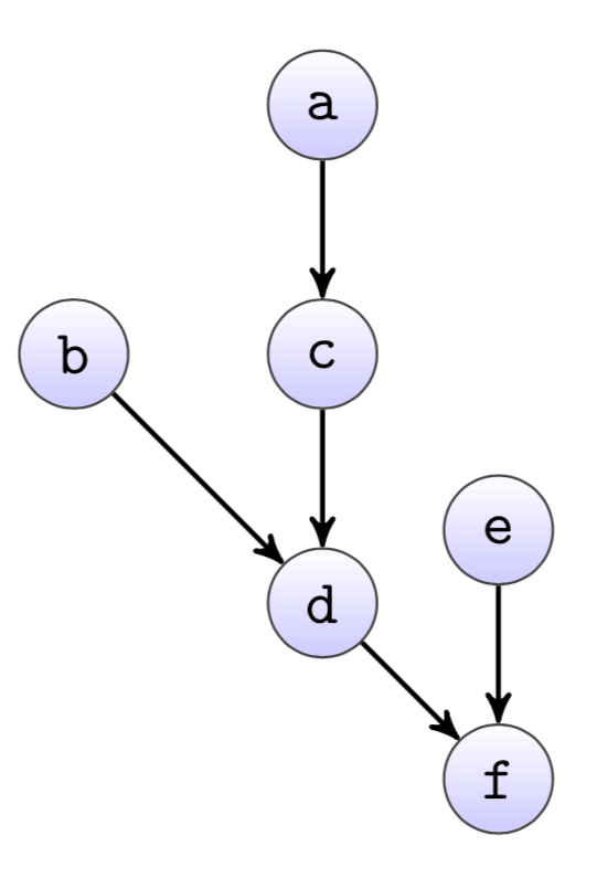
Given that individual jobs can have quite a different runtime, the best possible order is usually not obvious from the dependency graph. Looking at the example dependency graph from, it may seem that job a should be the first to run, followed by jobs b and c.
However, it is quite easy to construct an example where this would not be a good choice, namely if job e takes much longer than the other jobs. Therefore, the job scheduler calculates cost-based priorities for all jobs, that define in which order they are run.
Technically, we calculate the longest path from each node to the sink of the graph, based on some cost measure. The cost measure is currently simply the average runtime over the last 30 days of a job. Priority of a job is then the sum of the cost from all nodes on the longest path from the node to the sink.
| Node | a |
b |
c |
d |
e |
f |
|---|---|---|---|---|---|---|
| Runtime | 10 | 30 | 10 | 5 | 50 | 10 |
| Runtime | 35 | 45 | 25 | 15 | 60 | 10 |
The table shows an example of runtimes for the graph from above and the resulting priorities. Jobs with higher priorities are run first, so the first job to run in this case would be e.
The dependency graph is directed and acyclic, so the priorities can be calculated with a breadth-first search starting from the sink.
graph = {
    'sink': 'f',
    'nodes': {
        'f': {'cost': 10, 'dependencies': ['d', 'e']},
        'e': {'cost': 50, 'dependencies': []},
        'd': {'cost': 5, 'dependencies': ['b', 'c']},
        'c': {'cost': 10, 'dependencies': ['a']},
        'b': {'cost': 30, 'dependencies': []},
        'a': {'cost': 10, 'dependencies': []}
    }
}

# Initialize priorities with own cost
priorities = {k: v['cost'] for k, v in graph['nodes'].items()}

# Breadth first search starting from the sink of the graph
nodes = [graph['sink']]
while nodes:
    next_level = []
    for node in nodes:
        for dependency in graph['nodes'][node]['dependencies']:
            # Update priority iff the current path is more expensive
            priorities[dependency] = max(priorities[dependency],
                                        priorities[node] + graph['nodes'][dependency]['cost'])
            next_level.append(dependency)
    nodes = next_level
The runtime of the scheduling algorithm doesn't matter much again, because the graph is by definition small. And because the graph is also directed and acyclic, the longest path can be calculated efficiently anyway.
The longest path with just the job runtime as cost measure is not really guaranteed to find the best possible solution, but nevertheless seems to work quite well in praxis. The cost measure may be improved by taking i.e. CPU and IO usage of a job into account, even though this is generally difficult to measure. Running a job that is CPU bound in parallel to another one that is IO bound is however certainly better than running two jobs that are both IO bound.
Generally, the scheduler does not take into account how parallel jobs influence each other, and also does not really optimize for overall runtime by comparing to previous runs.
The average runtime may be calculated with a stronger influence for more recent runtimes, to adapt more quickly to changing runtimes.
