Five years of Weight Tracking
After I moved back from New Jersey in June 2008 I started to track my body weight more seriously. My routine usually consists of getting up and after finishing the morning bathroom I would step on my scale. That way I try to ensure that the condition for each weighing are as similar as possible. I recorded my weight on paper and eventually would put everything into a spreadsheet for further analysis.
In January 2011 I upgraded my bathroom scale to the Withings WiFi Body Scale. That way I could automate the process of tracking my weight by just stepping on it. No more writing on paper and eventually transferring everything into spreadsheets.
The people at Withings provide an API so external services could access your weight data. A nice way to get better charts is through Trendweight. Just link your Withings account to the web site and they will generate nice JavaScript charts of your weight/body fat/lean mass. Another great feature is the export functionality where you can export a comma separated version of your data including trend values for total weight as well as fat %, fat mass, and lean mass.
Using the exported data we can fire up R to look at the data:
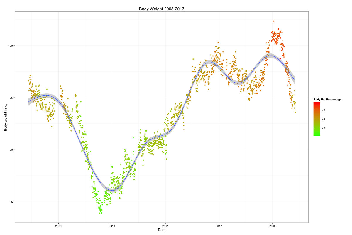
The generated chart shows my weight loss in 2009, where I started cycling again after years of absence. From my lowest in the Fall of 2009 I gradually gained weight throughout 2010, 2011 until 2012, where I hit the 100 kg mark around Christmas time:

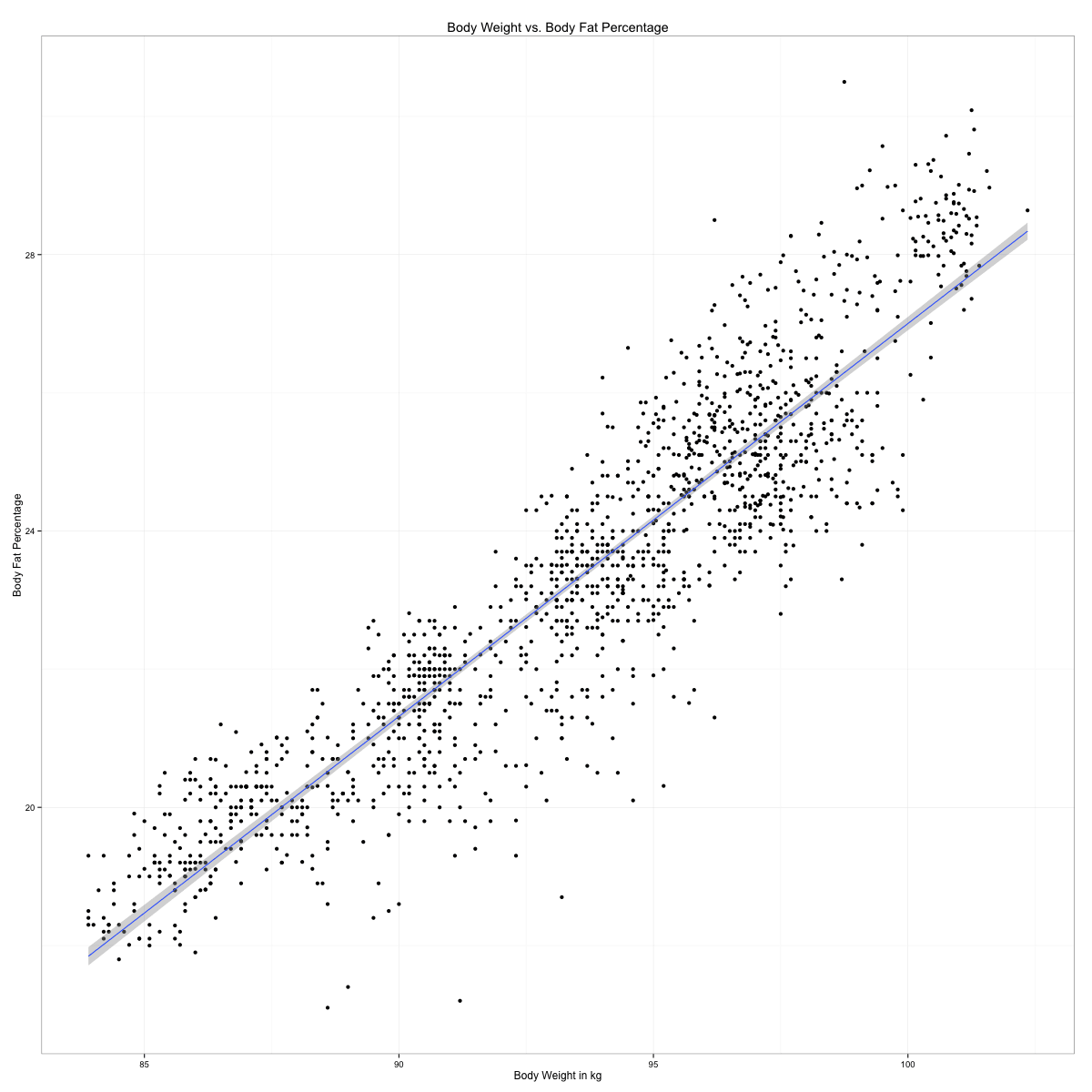
That was enough and I decided it was time to start working out again. So far, I am at a good downwards trend. I have to keep up that momentum. My next goal is to get between 80 kg and 85 kg and then maintain my weight. The color of the dots reflect my body fat percentage and there seems to be a strong correlation between body fat and my actual weight:

Doing a simple linear regression gives us an adjusted R-squared of 0.8419